
吴恩达深度学习 C2_W1_Assignment
任务1:初始化指定权重
Part0:准备数据
1 | import numpy as np |

我们需要一个分类器来区分蓝点和红点。
Part1:神经网络模型
如下已有一个三层神经网络,并尝试以下三种方法:
- Zeros initialization
- Random initialization
- He initialization
1 | def model(X, Y, learning_rate = 0.01, num_iterations = 15000, print_cost = True, initialization = "he"): |
Exercise1:Zero initialization
将以下参数初始化为0:
- the weight matrices (𝑊[1],𝑊[2],𝑊[3],…,𝑊[𝐿−1],𝑊[𝐿])
- the bias vectors (𝑏[1],𝑏[2],𝑏[3],…,𝑏[𝐿−1],𝑏[𝐿])
1 | def initialize_parameters_zeros(layers_dims): |
我们迭代15000次训练模型,观察结果:
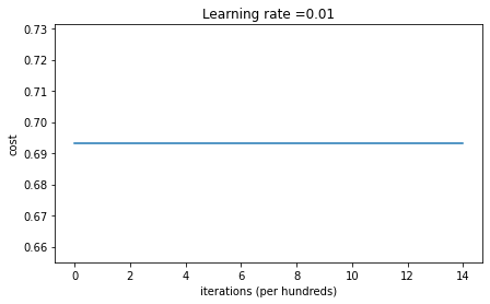
1 | On the train set: |
我们可以看出性能非常差,成本没有真正降低,我们来可视化一下分类结果:
1 | plt.title("Model with Zeros initialization") |

我们可以看出该模型预测每个示例均为0。一般来说,所有权重初始化为0会导致网络无法打破对称性,这意味着每一层的每一个神经元将学习相同的东西。
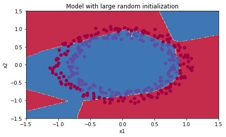
Exercise2:Random initialization
为了打破对称性,我们需要随机初始化权重。
1 | def initialize_parameters_random(layers_dims): |
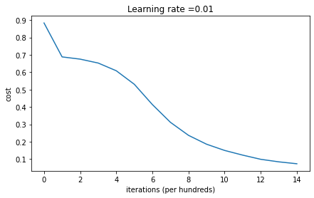
同样的,我们来观察一下迭代15000后的效果:
1 | On the train set: |
可以看到,我们得到了比之前更好的结果。同样的,我们来可视化一下分类效果:
1 | plt.title("Model with large random initialization") |
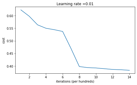
Exercise3:He initialization
初始化W时,乘以$\sqrt{\frac{2}{\text{dimension of the previous layer}}}$
1 | def initialize_parameters_he(layers_dims): |
同样的,我们来观察一下迭代15000后的效果:
1 | On the train set: |
观察一下分类效果:
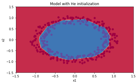
可以看出,He initialization很好的进行了分类。
任务2:在深度学习模型中使用正则化
Part0:库的准备
1 | # import packages |
问题描述:推荐法国队守门员踢球的位置,这样法国的球员就可以头击球了

数据为法国过去十场比赛的2D数据集:
1 | train_X, train_Y, test_X, test_Y = load_2D_dataset() |

每个点对应于足球场上的一个位置,如果圆点是蓝色的,说明法国选手设法用头击球。如果为红色,则表示对方球员用头击球。
我们的目标为:找出守门员应该在球场上踢球的位置。
Part1:使用非正则化的模型
1 | def model(X, Y, learning_rate = 0.3, num_iterations = 30000, print_cost = True, lambd = 0, keep_prob = 1): |
我们在不进行任何正则化的情况下训练模型,并在训练/测试集上观察精度
1 | parameters = model(train_X, train_Y) |

1 | On the training set: |
观察一下决策边界:
1 | plt.title("Model without regularization") |

可以看出,此模型过度拟合了训练集,接下来我们来看两种减少过度装配的技术。
Exercise1:L2 Regularization
代价函数如下:
1 | def compute_cost_with_regularization(A3, Y, parameters, lambd): |
Exercise2:实现有正则化后的反向传播
1 | def backward_propagation_with_regularization(X, Y, cache, lambd): |
现在让我们使用L2正则化来运行模型,观察效果:
1 | parameters = model(train_X, train_Y, lambd = 0.7) |

1 | On the train set: |
可以看出,测试集的准确率提高了,让我们绘制一下决策边界:
1 | plt.title("Model with L2-regularization") |

- $\lambda$是一个超参数,可以通过验证集进行调整
- L2正则化使决策边界更加平滑,如果$\lambda$太大,也可能过平滑,导致模型具有高偏差。
Exercise3:实现带有dropout的前向传播
在每次迭代中,通过𝑘𝑒𝑒𝑝_𝑝𝑟𝑜𝑏来控制关闭神经元的概率。Dropout背后的想法是,在每一次迭代中,训练一个只使用神经元的一个子集的的不同模型,这样,神经元对一个特定神经元的激活就会变的不那么敏感。
步骤如下:
- 创建一个和$A^{[1]}$具有相同维度的矩阵$D^{[1]} = [d^{1} d^{1} … d^{1}]$
- 通过𝑘𝑒𝑒𝑝_𝑝𝑟𝑜𝑏来对矩阵$D^{[1]}$赋值
- 将A矩阵与D矩阵相乘,起到关闭神经元的作用
- 将$A^{[1]}$除以𝑘𝑒𝑒𝑝_𝑝𝑟𝑜𝑏,确保结果仍然具有没有dropout时相同的预期值。
1 | def forward_propagation_with_dropout(X, parameters, keep_prob = 0.5): |
Exercise4:实现带有dropout的反向传播
步骤如下:
- 我们曾在前向传播中使用mask关闭了一些神经元。所以在反向传播中,我们需要关闭相同的神经元。
- 在前向传播中,我们将
A1除以keep_prob,因此,在反向传播中,我们需要将dA1除以keep_prob。
1 | def backward_propagation_with_dropout(X, Y, cache, keep_prob): |
现在让我们来运行带有dropout的模型,观察效果:
1 | parameters = model(train_X, train_Y, keep_prob = 0.86, learning_rate = 0.3) |
1 | On the train set: |
很遗憾,我做出来的结果与预期结果不符,测试集的准确率并没有达到预期的95%。
观察一下决策边界:
1 | plt.title("Model with dropout") |

总结:
- 正则化能帮助我们减少过度拟合
- 正则化能使权重降低
任务3:实现和使用梯度检查
Part0:库的准备
1 | # Packages |
梯度检查是如何运行的?
我们先回顾一下导数(梯度)的定义:
我们需要做的便是确保这个值是正确的。
Exercise1:一维梯度检测
考虑一维线性函数$J(\theta) = \theta x$,我们将计算$J()$和导数$\frac{\partial J}{\partial \theta}$,然后再使用梯度检测确保$J()$是正确的。

下面来实现它的前向传播和反向传播:
1 | def forward_propagation(x, theta): |
1 | def backward_propagation(x, theta): |
实现梯度检测的步骤如下:
- 计算gradapprox
- $\theta^{+} = \theta + \varepsilon$
- $\theta^{-} = \theta - \varepsilon$
- $J^{+} = J(\theta^{+})$
- $J^{-} = J(\theta^{-})$
- $gradapprox = \frac{J^{+} - J^{-}}{2 \varepsilon}$
- 然后使用反向传播计算梯度
- 最后,计算相对差值:$difference = \frac {\mid\mid grad - gradapprox \mid\mid_2}{\mid\mid grad \mid\mid_2 + \mid\mid gradapprox \mid\mid_2}$
tip:
- 计算范数时使用
np.linalg.norm(...)
1 | def gradient_check(x, theta, epsilon = 1e-7): |
Exercise2:N维梯度检测

实现前向传播和反向传播:
1 | def forward_propagation_n(X, Y, parameters): |
1 | def backward_propagation_n(X, Y, cache): |
导数公式仍然为:
但是由于$\theta$不再是标量,而是一个字典,所以已经提前准备好了一个函数dictionary_to_vector() ,将所有参数重塑为向量并进行连接。同时还有反函数vector_to_dictionary()。

计算步骤:
- 计算
J_plus[i]:- Set $\theta^{+}$ to
np.copy(parameters_values) - Set $\theta^{+}_i$ to $\theta^{+}_i + \varepsilon$
- 使用
forward_propagation_n(x, y, vector_to_dictionary( 𝜃+ ))计算$J^{+}_i$
- Set $\theta^{+}$ to
- 同样的方法计算
J_minus[i] - 计算$gradapprox[i] = \frac{J^{+}_i - J^{-}_i}{2 \varepsilon}$
- 计算$difference = \frac {| grad - gradapprox |_2}{| grad |_2 + | gradapprox |_2 }$
1 | def gradient_check_n(parameters, gradients, X, Y, epsilon = 1e-7): |