吴恩达深度学习 C2_W2_Assignment
任务:优化方法
Part0:库的准备
1 | import numpy as np |
Part1:梯度下降
Exercise1:实现梯度下降
1 | def update_parameters_with_gd(parameters, grads, learning_rate): |
1.1 随机梯度下降

从上图可以看出,SGD经过多次振荡达到收敛,但是它的每一步都比GD快。
在实践中,我们可以使用小批量梯度下降,会导致更快的优化

- 以上三种方法的区别在于执行一个更新步骤的示例数量。
1.2 小批量梯度下降
让我们来学习一下如何从训练集(X, Y) 中构建小批量。
Shuffle:

分区:
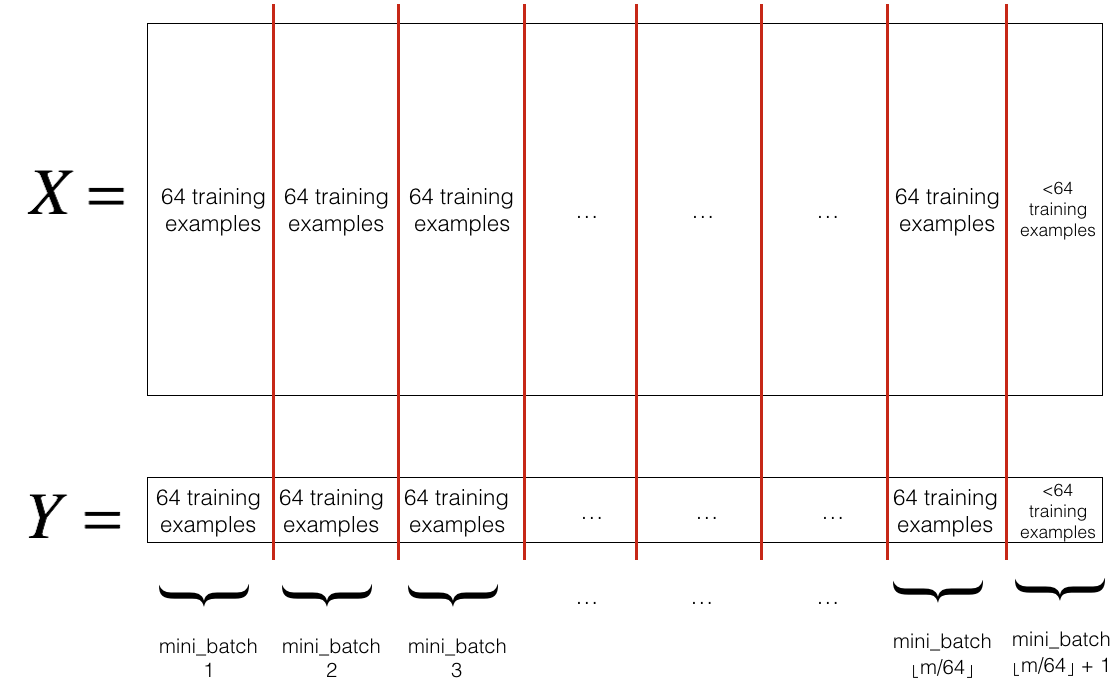
Exercise2:实现随机小批量
1
2
3
4
5
6
7
8
9
10
11
12
13
14
15
16
17
18
19
20
21
22
23
24
25
26
27
28
29
30
31
32
33
34
35
36
37
38
39
40
41
42
43
44# GRADED FUNCTION: random_mini_batches
def random_mini_batches(X, Y, mini_batch_size = 64, seed = 0):
"""
Creates a list of random minibatches from (X, Y)
Arguments:
X -- input data, of shape (input size, number of examples)
Y -- true "label" vector (1 for blue dot / 0 for red dot), of shape (1, number of examples)
mini_batch_size -- size of the mini-batches, integer
Returns:
mini_batches -- list of synchronous (mini_batch_X, mini_batch_Y)
"""
np.random.seed(seed)
m = X.shape[1] # number of training examples
mini_batches = []
# Step 1: Shuffle (X, Y)
permutation = list(np.random.permutation(m))
shuffled_X = X[:, permutation]
shuffled_Y = Y[:, permutation].reshape((1,m))
# Step 2: Partition (shuffled_X, shuffled_Y). Minus the end case.
num_complete_minibatches = math.floor(m/mini_batch_size) # number of mini batches of size mini_batch_size in your partitionning
for k in range(0, num_complete_minibatches):
### START CODE HERE ### (approx. 2 lines)
mini_batch_X = shuffled_X[:, k * mini_batch_size: (k + 1) * mini_batch_size]
mini_batch_Y = shuffled_Y[:, k * mini_batch_size: (k + 1) * mini_batch_size]
### END CODE HERE ###
mini_batch = (mini_batch_X, mini_batch_Y)
mini_batches.append(mini_batch)
# Handling the end case (last mini-batch < mini_batch_size)
if m % mini_batch_size != 0:
### START CODE HERE ### (approx. 2 lines)
mini_batch_X = shuffled_X[:, num_complete_minibatches * mini_batch_size: ]
mini_batch_Y = shuffled_Y[:, num_complete_minibatches * mini_batch_size: ]
### END CODE HERE ###
mini_batch = (mini_batch_X, mini_batch_Y)
mini_batches.append(mini_batch)
return mini_batchesPart2:Momentum(动量)
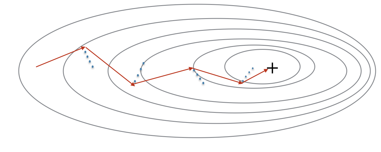
动量考虑过去的梯度以平滑更新
- 红色箭头表示下降一步所采取的方向
- 蓝色的点表示每一步渐变的方向
Exercise3:初始化速度
1
2
3
4
5
6
7
8
9
10
11
12
13
14
15
16
17
18
19
20
21
22
23
24
25
26
27
def initialize_velocity(parameters):
"""
Initializes the velocity as a python dictionary with:
- keys: "dW1", "db1", ..., "dWL", "dbL"
- values: numpy arrays of zeros of the same shape as the corresponding gradients/parameters.
Arguments:
parameters -- python dictionary containing your parameters.
parameters['W' + str(l)] = Wl
parameters['b' + str(l)] = bl
Returns:
v -- python dictionary containing the current velocity.
v['dW' + str(l)] = velocity of dWl
v['db' + str(l)] = velocity of dbl
"""
L = len(parameters) // 2 # number of layers in the neural networks
v = {}
# Initialize velocity
for l in range(L):
### START CODE HERE ### (approx. 2 lines)
v['dW' + str(l + 1)] = np.zeros_like(parameters['W' + str(l + 1)])
v['db' + str(l + 1)] = np.zeros_like(parameters['b' + str(l + 1)])
### END CODE HERE ###
return vExercise4:使用动量实现参数更新
- L为层数
- $\beta$为动量
- $\alpha$为学习率
1
2
3
4
5
6
7
8
9
10
11
12
13
14
15
16
17
18
19
20
21
22
23
24
25
26
27
28
29
30
31
32
33
34
35
36
37def update_parameters_with_momentum(parameters, grads, v, beta, learning_rate):
"""
Update parameters using Momentum
Arguments:
parameters -- python dictionary containing your parameters:
parameters['W' + str(l)] = Wl
parameters['b' + str(l)] = bl
grads -- python dictionary containing your gradients for each parameters:
grads['dW' + str(l)] = dWl
grads['db' + str(l)] = dbl
v -- python dictionary containing the current velocity:
v['dW' + str(l)] = ...
v['db' + str(l)] = ...
beta -- the momentum hyperparameter, scalar
learning_rate -- the learning rate, scalar
Returns:
parameters -- python dictionary containing your updated parameters
v -- python dictionary containing your updated velocities
"""
L = len(parameters) // 2 # number of layers in the neural networks
# Momentum update for each parameter
for l in range(L):
### START CODE HERE ### (approx. 4 lines)
# compute velocities
v['dW' + str(l + 1)] = beta * v['dW' + str(l + 1)] + (1 - beta) * grads['dW' + str(l + 1)]
v['db' + str(l + 1)] = beta * v['db' + str(l + 1)] + (1 - beta) * grads['db' + str(l + 1)]
# update parameters
parameters['W' + str(l + 1)] -= learning_rate * v['dW' + str(l + 1)]
parameters['b' + str(l + 1)] -= learning_rate * v['db' + str(l + 1)]
### END CODE HERE ###
return parameters, v- $\beta$越大,更新就越平稳,考虑过去的梯度就越多,但是$\beta$太大,就可能会使更新过多
- $\beta$=0.9通常为合理的默认值
Part3:Adam
Adam结合了RMSProp和Momentum的想法
- 它计算过去梯度的指数加权平均值,并存储在$v$(before bias correction) and $v^{corrected}$(with bias correction)中。
- 它计算过去梯度平方的指数加权平均值,并存储在$s$(before bias correction) and $s^{corrected}$(with bias correction)中。
更新规则如下:
Exercise5:初始化Adam变量
1
2
3
4
5
6
7
8
9
10
11
12
13
14
15
16
17
18
19
20
21
22
23
24
25
26
27
28
29
30
31
32
33
34
35def initialize_adam(parameters) :
"""
Initializes v and s as two python dictionaries with:
- keys: "dW1", "db1", ..., "dWL", "dbL"
- values: numpy arrays of zeros of the same shape as the corresponding gradients/parameters.
Arguments:
parameters -- python dictionary containing your parameters.
parameters["W" + str(l)] = Wl
parameters["b" + str(l)] = bl
Returns:
v -- python dictionary that will contain the exponentially weighted average of the gradient.
v["dW" + str(l)] = ...
v["db" + str(l)] = ...
s -- python dictionary that will contain the exponentially weighted average of the squared gradient.
s["dW" + str(l)] = ...
s["db" + str(l)] = ...
"""
L = len(parameters) // 2 # number of layers in the neural networks
v = {}
s = {}
# Initialize v, s. Input: "parameters". Outputs: "v, s".
for l in range(L):
### START CODE HERE ### (approx. 4 lines)
v["dW" + str(l + 1)] = np.zeros_like(parameters["W" + str(l + 1)])
v["db" + str(l + 1)] = np.zeros_like(parameters["b" + str(l + 1)])
s["dW" + str(l + 1)] = np.zeros_like(parameters["W" + str(l + 1)])
s["db" + str(l + 1)] = np.zeros_like(parameters["b" + str(l + 1)])
### END CODE HERE ###
return v, sExercise6:实现参数更新
1
2
3
4
5
6
7
8
9
10
11
12
13
14
15
16
17
18
19
20
21
22
23
24
25
26
27
28
29
30
31
32
33
34
35
36
37
38
39
40
41
42
43
44
45
46
47
48
49
50
51
52
53
54
55
56
57
58
59
60
61
62def update_parameters_with_adam(parameters, grads, v, s, t, learning_rate = 0.01,
beta1 = 0.9, beta2 = 0.999, epsilon = 1e-8):
"""
Update parameters using Adam
Arguments:
parameters -- python dictionary containing your parameters:
parameters['W' + str(l)] = Wl
parameters['b' + str(l)] = bl
grads -- python dictionary containing your gradients for each parameters:
grads['dW' + str(l)] = dWl
grads['db' + str(l)] = dbl
v -- Adam variable, moving average of the first gradient, python dictionary
s -- Adam variable, moving average of the squared gradient, python dictionary
learning_rate -- the learning rate, scalar.
beta1 -- Exponential decay hyperparameter for the first moment estimates
beta2 -- Exponential decay hyperparameter for the second moment estimates
epsilon -- hyperparameter preventing division by zero in Adam updates
Returns:
parameters -- python dictionary containing your updated parameters
v -- Adam variable, moving average of the first gradient, python dictionary
s -- Adam variable, moving average of the squared gradient, python dictionary
"""
L = len(parameters) // 2
v_corrected = {} # Initializing first moment estimate, python dictionary
s_corrected = {} # Initializing second moment estimate, python dictionary
# Perform Adam update on all parameters
for l in range(L):
# Moving average of the gradients. Inputs: "v, grads, beta1". Output: "v".
### START CODE HERE ### (approx. 2 lines)
v["dW" + str(l + 1)] = beta1 * v["dW" + str(l + 1)] + (1 - beta1) * grads["dW" + str(l + 1)]
v["db" + str(l + 1)] = beta1 * v["db" + str(l + 1)] + (1 - beta1) * grads["db" + str(l + 1)]
### END CODE HERE ###
# Compute bias-corrected first moment estimate. Inputs: "v, beta1, t". Output: "v_corrected".
### START CODE HERE ### (approx. 2 lines)
v_corrected["dW" + str(l + 1)] = v["dW" + str(l + 1)] / (1 - beta1 ** t)
v_corrected["db" + str(l + 1)] = v["db" + str(l + 1)] / (1 - beta1 ** t)
### END CODE HERE ###
# Moving average of the squared gradients. Inputs: "s, grads, beta2". Output: "s".
### START CODE HERE ### (approx. 2 lines)
s["dW" + str(l + 1)] = beta2 * s["dW" + str(l + 1)] + (1 - beta2) * np.multiply(grads["dW" + str(l + 1)], grads["dW" + str(l + 1)])
s["db" + str(l + 1)] = beta2 * s["db" + str(l + 1)] + (1 - beta2) * np.multiply(grads["db" + str(l + 1)], grads["db" + str(l + 1)])
### END CODE HERE ###
# Compute bias-corrected second raw moment estimate. Inputs: "s, beta2, t". Output: "s_corrected".
### START CODE HERE ### (approx. 2 lines)
s_corrected["dW" + str(l + 1)] = s["dW" + str(l + 1)] / (1 - beta2 ** t)
s_corrected["db" + str(l + 1)] = s["db" + str(l + 1)] / (1 - beta2 ** t)
### END CODE HERE ###
# Update parameters. Inputs: "parameters, learning_rate, v_corrected, s_corrected, epsilon". Output: "parameters".
### START CODE HERE ### (approx. 2 lines)
parameters['W' + str(l + 1)] -= learning_rate * v_corrected["dW" + str(l + 1)] / (epsilon + np.sqrt(s_corrected["dW" + str(l + 1)]))
parameters['b' + str(l + 1)] -= learning_rate * v_corrected["db" + str(l + 1)] / (epsilon + np.sqrt(s_corrected["db" + str(l + 1)]))
### END CODE HERE ###
return parameters, v, sPart4:采用不同优化算法的模型
先来看看数据集
1
train_X, train_Y = load_dataset()

定义模型:
1
2
3
4
5
6
7
8
9
10
11
12
13
14
15
16
17
18
19
20
21
22
23
24
25
26
27
28
29
30
31
32
33
34
35
36
37
38
39
40
41
42
43
44
45
46
47
48
49
50
51
52
53
54
55
56
57
58
59
60
61
62
63
64
65
66
67
68
69
70
71
72
73
74
75
76
77
78
79
80
81
82
83def model(X, Y, layers_dims, optimizer, learning_rate = 0.0007, mini_batch_size = 64, beta = 0.9,
beta1 = 0.9, beta2 = 0.999, epsilon = 1e-8, num_epochs = 10000, print_cost = True):
"""
3-layer neural network model which can be run in different optimizer modes.
Arguments:
X -- input data, of shape (2, number of examples)
Y -- true "label" vector (1 for blue dot / 0 for red dot), of shape (1, number of examples)
layers_dims -- python list, containing the size of each layer
learning_rate -- the learning rate, scalar.
mini_batch_size -- the size of a mini batch
beta -- Momentum hyperparameter
beta1 -- Exponential decay hyperparameter for the past gradients estimates
beta2 -- Exponential decay hyperparameter for the past squared gradients estimates
epsilon -- hyperparameter preventing division by zero in Adam updates
num_epochs -- number of epochs
print_cost -- True to print the cost every 1000 epochs
Returns:
parameters -- python dictionary containing your updated parameters
"""
L = len(layers_dims) # number of layers in the neural networks
costs = [] # to keep track of the cost
t = 0 # initializing the counter required for Adam update
seed = 10 # For grading purposes, so that your "random" minibatches are the same as ours
# Initialize parameters
parameters = initialize_parameters(layers_dims)
# Initialize the optimizer
if optimizer == "gd":
pass # no initialization required for gradient descent
elif optimizer == "momentum":
v = initialize_velocity(parameters)
elif optimizer == "adam":
v, s = initialize_adam(parameters)
# Optimization loop
for i in range(num_epochs):
# Define the random minibatches. We increment the seed to reshuffle differently the dataset after each epoch
seed = seed + 1
minibatches = random_mini_batches(X, Y, mini_batch_size, seed)
for minibatch in minibatches:
# Select a minibatch
(minibatch_X, minibatch_Y) = minibatch
# Forward propagation
a3, caches = forward_propagation(minibatch_X, parameters)
# Compute cost
cost = compute_cost(a3, minibatch_Y)
# Backward propagation
grads = backward_propagation(minibatch_X, minibatch_Y, caches)
# Update parameters
if optimizer == "gd":
parameters = update_parameters_with_gd(parameters, grads, learning_rate)
elif optimizer == "momentum":
parameters, v = update_parameters_with_momentum(parameters, grads, v, beta, learning_rate)
elif optimizer == "adam":
t = t + 1 # Adam counter
parameters, v, s = update_parameters_with_adam(parameters, grads, v, s,
t, learning_rate, beta1, beta2, epsilon)
# Print the cost every 1000 epoch
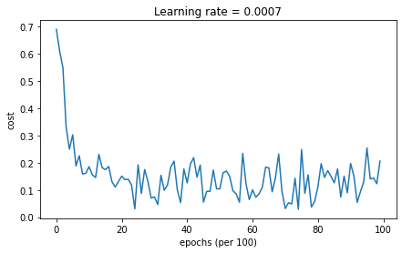
if print_cost and i % 1000 == 0:
print ("Cost after epoch %i: %f" %(i, cost))
if print_cost and i % 100 == 0:
costs.append(cost)
# plot the cost
plt.plot(costs)
plt.ylabel('cost')
plt.xlabel('epochs (per 100)')
plt.title("Learning rate = " + str(learning_rate))
plt.show()
return parameters4.1 小批量梯度下降
1
2
3
4
5
6
7
8
9
10
11
12
13
# train 3-layer model
layers_dims = [train_X.shape[0], 5, 2, 1]
parameters = model(train_X, train_Y, layers_dims, optimizer = "gd")
# Predict
predictions = predict(train_X, train_Y, parameters)
# Plot decision boundary
plt.title("Model with Gradient Descent optimization")
axes = plt.gca()
axes.set_xlim([-1.5,2.5])
axes.set_ylim([-1,1.5])
plot_decision_boundary(lambda x: predict_dec(parameters, x.T), train_X, train_Y)观察一下结果:

Accuracy: 0.7966666666666666

4.2 带动量的小批量梯度下降
1
2
3
4
5
6
7
8
9
10
11
12
13
# train 3-layer model
layers_dims = [train_X.shape[0], 5, 2, 1]
parameters = model(train_X, train_Y, layers_dims, beta = 0.9, optimizer = "momentum")
# Predict
predictions = predict(train_X, train_Y, parameters)
# Plot decision boundary
plt.title("Model with Momentum optimization")
axes = plt.gca()
axes.set_xlim([-1.5,2.5])
axes.set_ylim([-1,1.5])
plot_decision_boundary(lambda x: predict_dec(parameters, x.T), train_X, train_Y)观察一下结果:

Accuracy: 0.7966666666666666

4.3 具有Adam模式的小型批处理
1
2
3
4
5
6
7
8
9
10
11
12
13
# train 3-layer model
layers_dims = [train_X.shape[0], 5, 2, 1]
parameters = model(train_X, train_Y, layers_dims, optimizer = "adam")
# Predict
predictions = predict(train_X, train_Y, parameters)
# Plot decision boundary
plt.title("Model with Adam optimization")
axes = plt.gca()
axes.set_xlim([-1.5,2.5])
axes.set_ylim([-1,1.5])
plot_decision_boundary(lambda x: predict_dec(parameters, x.T), train_X, train_Y)观察一下结果:
Accuracy: 0.94